ggplot линия и сегмент Наполните

Question

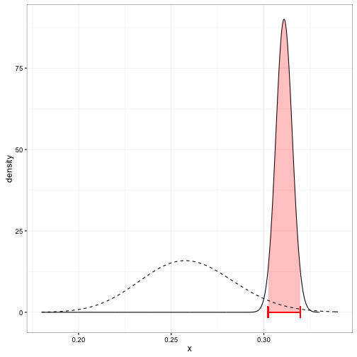
Я ищу, чтобы создать сюжет, который похож на this one on David Robinson's variance explained blog:

Я думаю, что я его для заливки, которая идет между заслуживающих доверия интервалами и под исключением задняя кривая. Если кто-нибудь знает, как это сделать, было бы здорово получить некоторые советы.

Вот некоторые примеры кода:

library(ebbr) 
library(ggplot2) 
library(dplyr) 

sample<- data.frame(id=factor(1:10), yes=c(20, 33, 44, 51, 50, 50, 66, 41, 91, 59), 
       total=rep(100, 10)) 

sample<- 
    sample %>% 
    mutate(rate=yes/total) 

pri<- 
    sample %>% 
    ebb_fit_prior(yes, total) 

sam.pri<- augment(pri, data=sample) 

post<- function(ID){ 
    a<- 
    sam.pri %>% 
    filter(id==ID) 

    ggplot(data=a, aes(x=rate))+ 
    stat_function(geom="line", col="black", size=1.1, fun=function(x) 
     dbeta(x, a$.alpha1, a$.beta1))+ 
    stat_function(geom="line", lty=2, size=1.1, 
        fun=function(x) dbeta(x, pri$parameters$alpha,  pri$parameters$beta))+ 
    geom_segment(aes(x=a$.low, y=0, xend=a$.low, yend=.5), col="red", size=1.05)+ 
    geom_segment(aes(x = a$.high, y=0, xend=a$.high, yend=.5), col="red", size=1.05)+ 
    geom_segment(aes(x=a$.low, y=.25, xend=a$.high, yend=.25), col="red", size=1.05)+ 
xlim(0,1) 
} 

post("10") 

Answer 1

я обычно делают это путем генерации данных для описания кривой вручную, добавляя нулевые значения Y для мин и макс заштрихованной области, и с помощью geom_polygon().

library(ebbr) 
library(ggplot2) 
library(dplyr) 

sample <- data.frame(id = factor(1:10), yes = c(20, 33, 44, 51, 50, 50, 66, 41, 91, 59), 
        total = rep(100, 10)) %>% 
    mutate(rate=yes/total) 

pri <- sample %>% 
    ebb_fit_prior(yes, total) 

sam.pri <- augment(pri, data = sample) 

a <- sam.pri %>% 
    filter(id == 10) 

# Make the x values for the shaded region 
x <- seq(from = a$.low, to = a$.high, length.out = 100) 

# Make the y values for the shaded region 
y <- dbeta(x, a$.alpha1, a$.beta1) 

# Make a data.frame for the shaded region, including zeroes 
shaded <- data.frame(x = c(x, a$.high, a$.low), y = c(y, 0, 0)) 

ggplot(data = a, aes(x = rate)) + 
    stat_function(geom = "line", col = "black", size = 1.1, 
       fun = function(x) dbeta(x, a$.alpha1, a$.beta1)) + 
    geom_polygon(data = shaded, aes(x, y), 
       fill = "red", alpha = 0.1) + 
    stat_function(geom = "line", lty = 2, size = 1.1, 
       fun = function(x) dbeta(x, pri$parameters$alpha,  pri$parameters$beta)) + 
    geom_segment(aes(x = a$.low, y = 0, xend = a$.low, yend = 0.5), col = "red", size = 1.05) + 
    geom_segment(aes(x = a$.high, y = 0, xend = a$.high, yend = .5), col = "red", size = 1.05) + 
    geom_segment(aes(x = a$.low, y = .25, xend = a$.high, yend = .25), col = "red", size = 1.05) + 
    xlim(0,1)